Graphing the performance of the market over the past 147 years.
Author’s note: I originally wrote this post in the fall of 2018 with the S&P 500 index at 2900.
The Longest Bull
This epic bull market made the news recently by taking out the previous high it had set in January of this year. It is also now being touted as the longest bull market in U.S. history. That latter bit is open to some debate depending on how you time your starting and ending points, but there is no denying that the U.S. market has had an impressive run since the depths of the Great Financial Crisis in 2009.
It seems an opportune time, then, to step back and try to put the current bull market into perspective. A picture is worth a thousand words, so let’s put together a graph of the US market going back 147 years, to see how this current bull stacks up against previous runs.
For this, I’ll be using the very generously provided data set found on Robert Shiller’s website.
In March of 2000, with impeccable timing, Robert Shiller released his now famous book, Irrational Exuberance, in which he argued convincingly that the market at the time was in an epic bubble. History proved him spectacularly right and to follow this up, in 2005 he released a second edition of his book with additional information on the brewing housing bubble, once again nailing it on the head. If he comes out with a third edition of his book anytime soon, we’d all better run for cover!
In his books, Shiller takes a close look at historical stock market performance and for this he put together a comprehensive database which included monthly average U.S. stock market prices going back all the way to 1871, along with information on dividends, earnings, inflation and interest rates. You can download all of this data, which he updates regularly, from his website.
This is an incredible treasure trove of data and I have spent countless hours playing around with it. For his data series, Shiller has spliced together several other discrete sets of data. He uses the S&P 500 as his marker of US stock performance over the past few decades. Before that, he uses what was then the more widely used S&P 90 index and before that he uses information collected by Cowles and Associates that they published in 1938 after painstakingly going through historical newspaper clippings, looking for references to stock prices, dividend announcements, etc. Clearly as you go further back in time, the data becomes increasingly unreliable. As well, markets have changed. In the late 1800’s, the market was made up mostly of railroad stocks with a few utilities and industrials sprinkled in for good measure. There were no multi billion dollar companies whose entire fate rested in the fickle thumbs of a group of smartphone-wielding pre-teens. The more things change, the more they stay the same, though, and I think we can still gain valuable insights by looking back at the full sweep of stock market history as the market has evolved over the past 147 years.
Before we get to graphing all this juicy data, let’s lay out some ground rules.
Dividends
First, we need to consider what it is we’re going to graph. Shiller reports the historical price level of the S&P 500. When you see in the newspaper that “the S&P just hit a new high today, closing at 2900”, that is what they are referring to. However, this price level is missing a key part of the puzzle: dividends. Most of the return from stocks over the past 147 years has actually come from the dividends they have paid out, not from the growth in the underlying share prices. Since 1871, stock prices have risen by 2.4% per year over and above the rate of inflation. Not exactly anything to write home about. However, if you include the dividends you would have received along the way, your annual rate of return rises to 6.9%. (Meaning that the average dividend yield was about 4.5% over this same time period) So when we’re graphing the long-term performance of the market, we need to factor dividends into the equation.
Inflation
Next, we need to make sure that we’ve properly accounted for the ravages of inflation. Here is a graph of the annual rate of growth in consumer prices over the preceding year and preceding 10 years. The 10-year version smooths out a lot of the noise from the annual series and gives a better sense of how inflation has waxed and waned over the years.
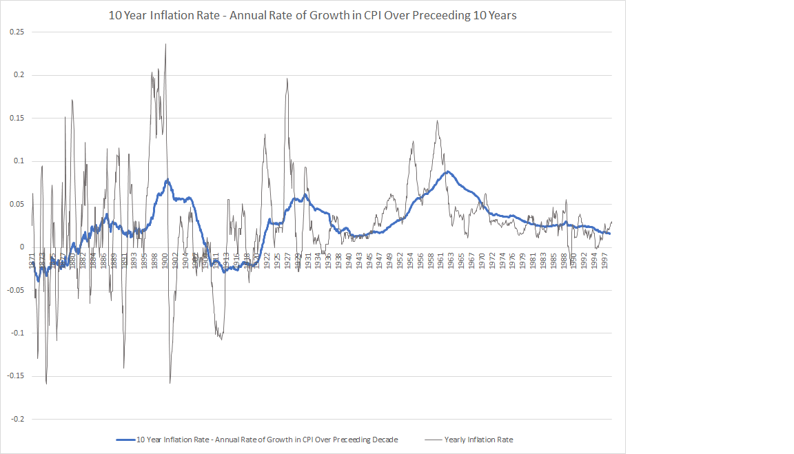
As you can see, inflation has periodically reared it’s ugly head, averaging 6-8% in the decades ending in 1920, 1950 and 1983. At other times, though, inflation was quite low or even non-existent. During the great depression prices actually fell by about 2% year over year.
These price changes can have quite an impact on the real rate of return you’d expect to get from the stock market. As an investor, if the market rises 5%, it is reasonable to expect that your own portfolio would also rise by 5%. However, if the price of everything else has risen by 10% in the meantime, then you’ve actually lost ground. The real rate of return of your investments has been negative 5%, not plus 5%.
When we graph out the performance of the market over the past 147 years, we need to take inflation into account. By subtracting the rate of inflation from the stock market’s performance every year we get the “real” inflation adjusted rate of return of the stock market. This more accurately reflects what an investor in the market would have actually achieved in practical terms and removes the distorting effect that periods of high inflation can have on long-term performance graphs.
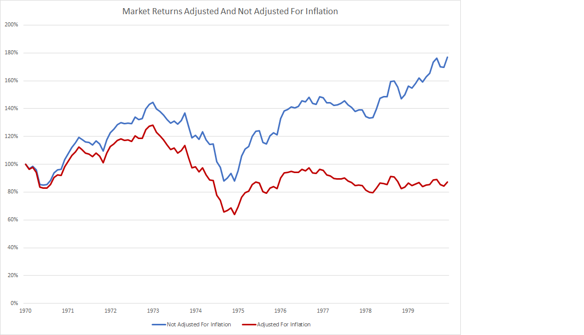
As an example, here is a graph of the market during the 70’s which was a period of high inflation and a terrible time for investors. The first graph shows the performance of the S&P 500 without making any adjustments for inflation. It doesn’t look half bad. There was a big hiccup along the way but over the decade, it looks like an investor would have made out fairly well, nearly doubling the value of their portfolio. However, consumer prices were skyrocketing over this time period and so in real, inflation adjusted terms, the investor’s portfolio would have bought a lot less at decade’s end than at the beginning. Adjusting our numbers for inflation gives a more accurate picture of what the investor would have really experienced during the decade.
Using Logarithms
Finally, we need to plot our results on a logarithmic scale. If we use a normal scale, changes in the early years get swamped by much larger changes, in absolute terms, in the later years. Here is a graph of the S&P 500 made without using a logarithmic scale…
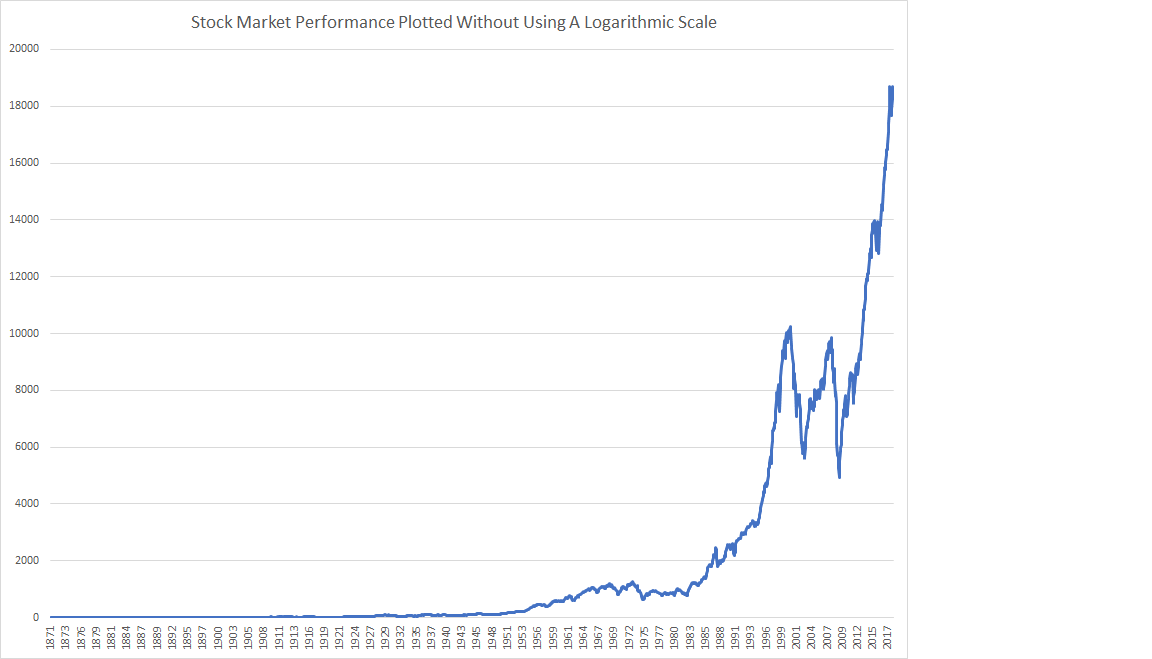
Not terribly informative is it?
Putting all of this together, then, what we’re interested in is the performance of the S&P 500 and its predecessor indexes over the past 147 years, with the dividend payouts along the way added in and with the results adjusted to factor in any loss of purchasing power as a result of inflation, all plotted on a logarithmic scale.
If we do all this, we get the following graph of the U.S. stock market, adjusted for inflation and dividends over the past century and a half…
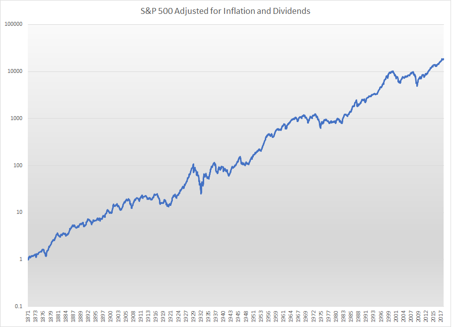
A reassuringly upward march when looked at over such a comprehensive period of time. Unfortunately, most investors’ time horizons are much shorter than 147 years so those stutters along the way are not quite as benign as they appear to be at first blush. One problem with a logarithmic scale is that it tends to visually squash everything together. Those drops in 1929, 1973, 2000 and 2007 were actually a lot scarier than they appear.
With stocks making new highs, it is worth pausing for a reality check and reminding ourselves of what bear markets, which have been a regular occurrence on Wall Street, look and feel like. Here is a close-up look at some of the worst bear markets of the past 147 years. I’ve chosen four situations in which prices (adjusted for inflation and dividends) ended the period no higher than when they began.
Bear Markets
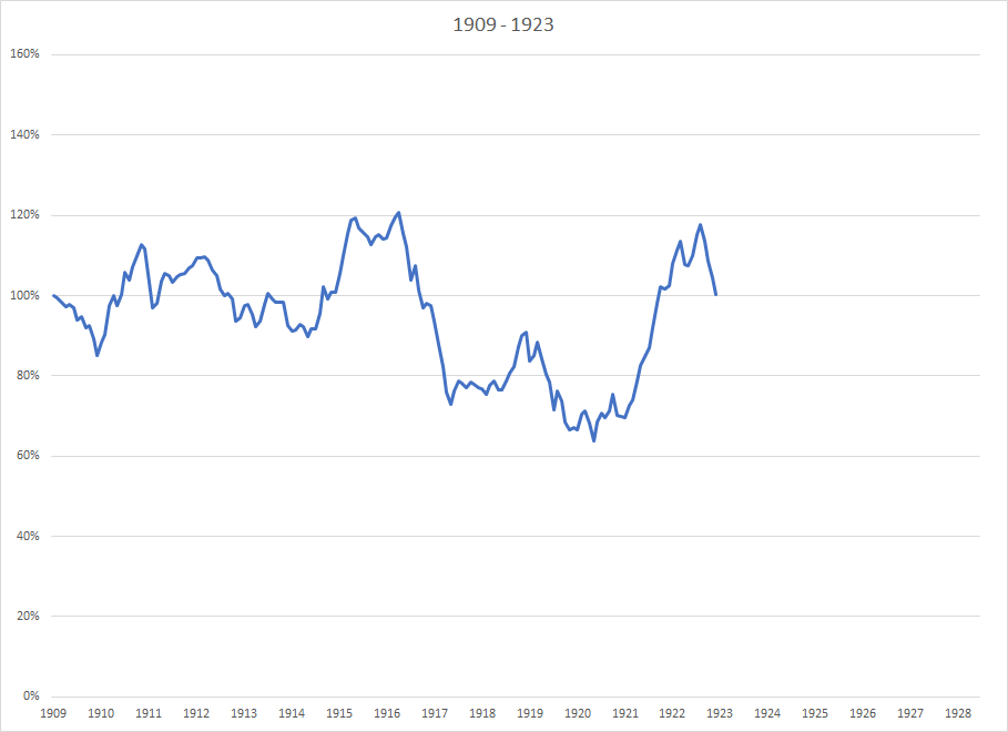
1909 – 1923
Stocks go nowhere for 14 years and suffer a 50% drop in the latter half of that time period as inflation spikes and Wall Street shuts down for 5 months during the first world war. A global flu pandemic likely didn’t help matters any.
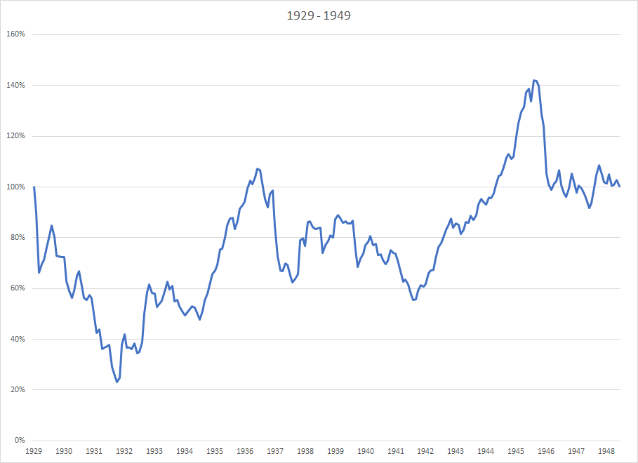
1929 – 1949
The great stock market crash of ’29 kicks things off with an almost 80% drop, peak to trough. If you had the resources and the fortitude to stay in the market, you would have recovered your losses within 7 years only to be hit again with another 40% drop in stock prices. Ultimately, by the end of the 20 year period, you were no further ahead than when you began.
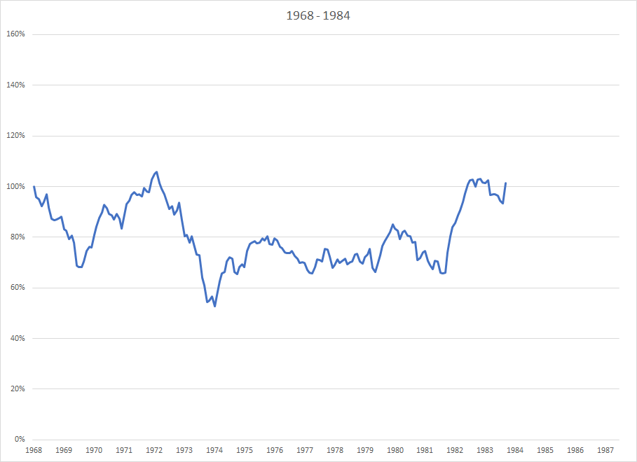
1968 – 1984
A great era for disco and classic rock. Not so much for stock market investors. Stagflation kept the market down for almost 16 years. When adjusted for the lost purchasing power caused by inflation, portfolios would have dropped in value by 30% in 1969/70 and then again by 50% in 1973/74. After the second walloping, they stayed down for the count for the next 8 years, only recovering back to where they began, 16 years earlier, in the early 80’s.
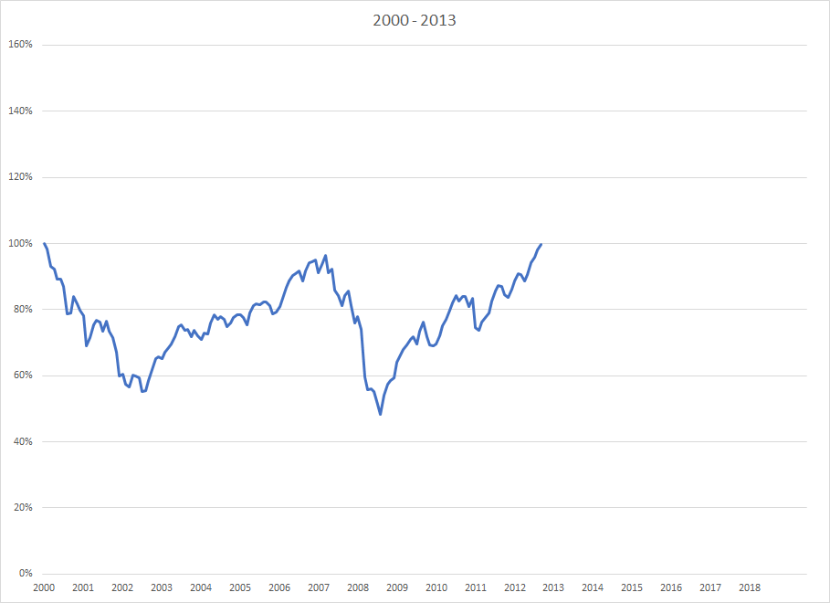
2000 – 2013
This one should still be fresh in most people’s memory although with the runup in prices of the last few years it is amazing how quickly we forget. First the dotcom implosion wiped 50% off stock prices and then, as soon as the market had managed to fight its way back up to breakeven, investors got hit with another 50% haircut. Overall, though, this was the shortest bear market of the four, clocking in at only 13 years and some would say there is still some unfinished business here.
Bull Markets
Using the guideposts I have arbitrarily set out here, it is worth noting that over the last 109 years, more than half the time has been spent in these bear markets. This should be enough to give investors sober second thoughts. However, the bull markets sandwiched in between these bear markets were quite spectacular times to be an investor and more than make up for the losses experienced during the bear maulings.
I’ve plotted the 4 bull markets that were interspersed with the bear markets above on the same graph. I’ve started each bull market at the point where the preceding bear market left off. As you can see from the graph, by this way of measuring things, the current bull market is a lightweight compared to the previous three.
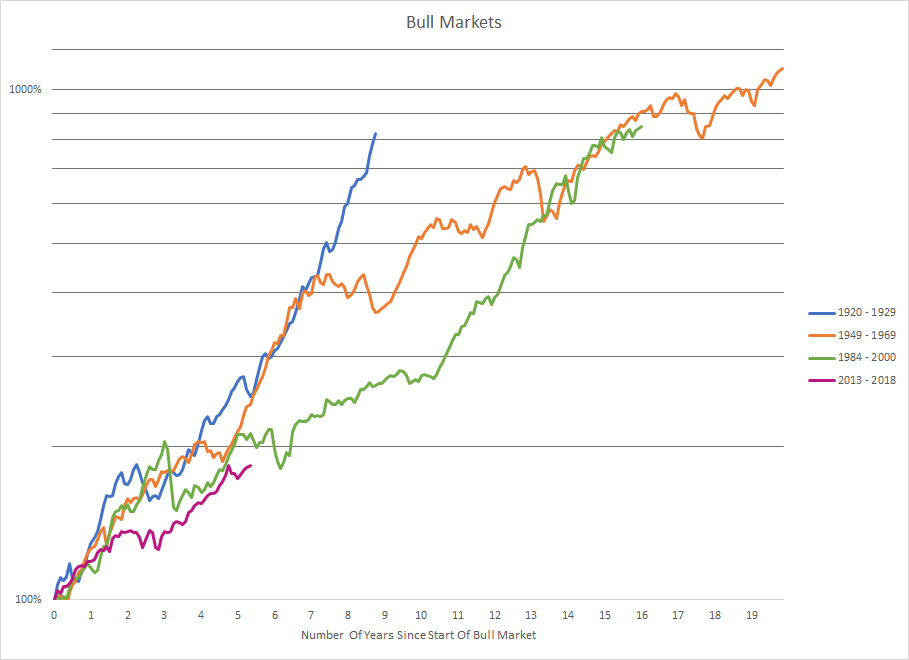
Far from being the longest bull market in US history, it is starting to look like the current bull market may just be getting started!
So can we all breath a deep sigh of relief and buy some more pot stocks? Well, not so fast. In order for stock prices to keep travelling along their merry way, the underlying earnings have to support that growth and the market’s price, relative to those earnings has to be supportive as well.
Ultimately, an investor’s returns are tied to the earnings of the companies he invests in. Those earnings may get paid out as dividends or could be used to buy back shares. Or, they could be used to re-invest in the business, generating future growth that way. While stock prices can move out of line with earnings for a time (and sometimes for many years at a time), ultimately they will always return to a level consistent with their underlying earnings.
The Caped Crusader
We can get a sense of this by graphing the p/e of the market over time. This is simply the ratio of the market index’s price to the aggregate earnings of the constituent stocks in the index. Robert Shiller, whose data I am using here, is probably best known for his popularisation of the CAPE index. CAPE stands for “cyclically adjusted p/e”. It’s a bit of a mouthful but the concept is very straight forward. The problem with using a regular p/e ratio is that earnings can bounce around quite a bit. During a recession, earnings often get depressed. Even though stock prices are also slumping, the p/e ratio can actually shoot up if earnings drop more than prices do. This makes a graph of the simple, trailing p/e ratio rather messy. What Shiller did was take the average of the last 10 year’s worth of earnings and use that, along with the current price, as the basis for his p/e. Using the 10 year average smooths out a lot of the noise and gives us a more useful yardstick.
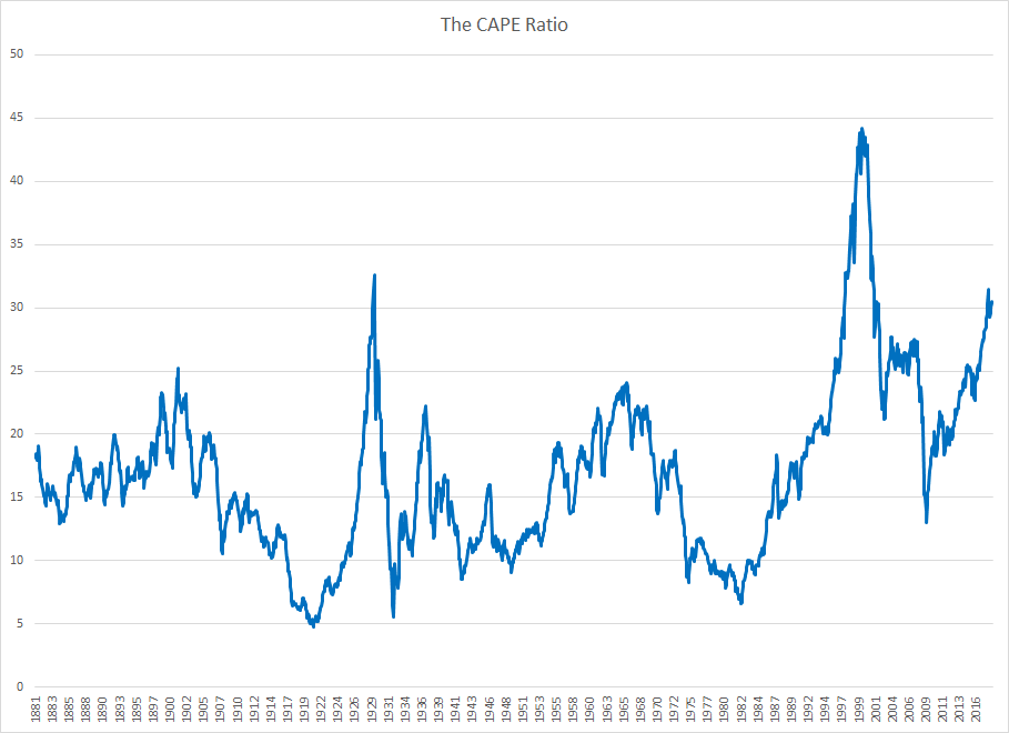
As you can see from this graph of the CAPE ratio over time, extremes in this ratio have correlated quite well with market tops and bottoms. We see high readings in 1929, 1937, 1966 and 2000, all years in which the market was at or near a top and was soon to experience a major drop. Likewise, we see low readings in 1920, 1932, 1982 and 2009, all years in which the market was about to turn around and start the next major bull run.
The big problem with extrapolating the current bull market forward is that this CAPE ratio is now much closer to the high levels it was at during previous market tops, just prior to a major drop than it is to the lower levels that would support a continuation of this bull run. Looking at my graph of the 4 superimposed bull markets (and using my method of dating those bull markets from the end of the preceding bear market, which in turn ends when the market finally definitively surpasses its previous highs), we see that by this methodology we are about 5 years into the current bull market. At a similar point in the other 3 bull markets of the past century, CAPE ratios were 14, 23 and 20. The CAPE ratio’s long-term average is 17. Currently the CAPE ratio is sitting at around 30, almost double what its long-term average has been and certainly above where it stood at similar points in the preceding 3 bull markets.
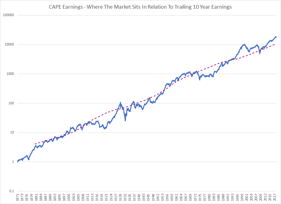
Another way to visualize this is to divide every point on our S&P 500 graph by the corresponding CAPE ratio on that date. This gives us what I’ll call the “CAPE earnings”. If we then multiply that number by the average CAPE over time of around 16.75 we get a nice visualization of how much above or below the historic average CAPE ratio the market is. Right now, the market has clearly moved above its long-term average and in fact, has been above that level for most of the last 20 years. The pessimists out there (including me) worry that at some point we’ll move to the opposite extreme and markets will trade well below their long-term average CAPE ratio. The transition from above average p/e ratios to below average p/e ratios could theoretically mean a drop of 50-75% in the market. As we’ve seen from our graphs of previous bear markets, that is not at all out of the question. Drops like that have happened many times in the past, often from overvalued levels like the present.
An Earnings Renaissance
While the chart above looks fairly worrisome, I have one final wrench to throw into the works. Yes, P/E ratios are high right now. At some point they are likely to go significantly lower. If that happens because the price part of the p/e equation drops, then we are in for a nasty bear market. But another possibility is that p/e ratios normalize, not because prices drop but because earnings surge upwards. This is not as far fetched a scenario as it seems. GDP growth has been quite weak in the aftermath of the Great Financial Crisis. In the past, periods of slow economic growth have sometimes been followed by catch up periods of significantly stronger growth. If the same thing were to happen going forward then earnings could move surprisingly higher. I personally don’t see this as the most likely outcome, especially considering current record high profit margins, high levels of corporate debt and an aging demographic, but you have to consider it as an outlier possibility. A burst of growth in underlying earnings, perhaps combined with a several year pause in the bull market could bring p/e ratios back into line and provide the fuel needed for this bull market to continue on for years to come.
There are a lot of moving parts to consider and predicting the future direction of the market is notoriously difficult. But studying past history is not a wasted effort. It shows us the range of possible outcomes and that range is far wider than most investors appreciate. Investors have had a roller coaster ride over the past 147 years. I’m sure the future will be equally hair-raising. Knowing what the past has delivered at least helps us prepare for an uncertain future. All we can do then is make sure we’re buckled in and try to enjoy the ride.
Authors’ note: It is now 6 years later, in the fall of 2024. Since I wrote this post, we’ve lived through a global pandemic, an extremely short-lived market crash that was brought to an abrupt halt by massive money printing and government stimulus, a global disruption in supply chains which contributed to an outbreak of inflation that lifted prices by over 20% and a war in Ukraine. We’ve experienced a bitcoin bubble, meme stock mania and are currently witnessing an artificial intelligence fueled frenzy. The pot stocks that were all the rage in 2018 are long forgotten. The market marches on its merry way and the S&P 500 is now at 5800. The CAPE ratio is at 37, still frighteningly high.